Chapter 18: Time Series Forecasting with AutoGluon
What you will learn
By the end of this chapter and its companion notebook, you will be able to:
Recognize when a research question is genuinely a forecasting problem
Format longitudinal or panel data for
TimeSeriesPredictorSet a forecast horizon and interpret quantile outputs with prediction intervals
Understand why temporal data leakage matters and how AutoGluon handles it for you
Some research datasets do not just describe a snapshot — they track how something changes over time. Repeated physiological measurements, weekly survey responses, yearly economic indicators, hourly sensor readings: all of these share a structure that tabular prediction is not designed for. When the goal is to predict future values based on past observations, the problem is called forecasting, and it calls for a different set of tools.
This chapter introduces TimeSeriesPredictor, AutoGluon’s forecasting module, using the same feasibility-testing philosophy from the tabular chapter. The goal is not to build a production forecasting system. It is to quickly find out whether there is enough temporal signal in your data to justify investing further, and to understand what the output is actually telling you [Shchur et al., 2023].
Is This a Forecasting Problem?
Not every dataset with a time column is a forecasting problem. This is worth pausing on before you write any code, because the answer shapes everything that follows.
A forecasting problem asks: given what I have observed up to now, what will the values look like at future time points? The output is a prediction over a future window.
But many research questions that involve time are not really asking that. A study comparing how two groups change over a six-week intervention period is usually asking a causal question, not a predictive one, and standard regression or mixed-effects models are the right tools. If your research question is “what will happen next” or “how much will we need,” then forecasting is appropriate. If it is “does X cause Y” or “how do groups differ,” forecasting is probably not the right frame.
If you decide forecasting is right for your problem, the next question is: over what horizon? That is a research decision, not a technical one. For a monthly health indicator, maybe you want a three-month-ahead forecast. For a sensor dataset, maybe 24 hours. TimeSeriesPredictor calls this prediction_length, and it is the first parameter you will set.
How Time Series Differs from Tabular Prediction
In tabular prediction, each row is an independent observation and the order of rows does not matter. In time series forecasting, the opposite is true. Rows are ordered, and the order is the whole point. The value at time t depends on values at t-1, t-2, and beyond.
This has one major consequence for how you evaluate your model: the train/test split must respect time. You train on earlier data and test on later data, never the reverse. A random split would let the model see future observations during training, which makes performance look unrealistically good. This is called temporal data leakage, and it is the most common pitfall in time series modeling [Hyndman and Athanasopoulos, 2021].
AutoGluon handles this correctly by default. You specify a forecast horizon, and it reserves the most recent prediction_length time steps of each series for validation. You do not need to manage the split yourself.
A second difference is the output format. Tabular prediction gives you a single predicted value per row. Time series forecasting gives you a distribution over future values at each step, specifically a set of quantiles (by default the 10th, 50th, and 90th percentiles). The 50th percentile is the point forecast; the others define a prediction interval. This is genuinely more useful for research because it forces you to communicate uncertainty rather than presenting a single number as ground truth.
Data Format: Getting Your Data into Shape
TimeSeriesPredictor expects data in long format, with three required columns [Shchur et al., 2023]:
Column |
Role |
Example values |
|---|---|---|
|
Unique identifier for each series |
|
|
Timestamp of the observation |
|
|
The value you want to forecast |
|
The “item” concept is important to understand. AutoGluon is designed for panel forecasting, meaning multiple related series measured over time. Each unique item_id is one series. If you are studying 50 patients and measuring heart rate weekly, each patient is one item. If you have only one location measuring air quality, you still have one item. Single-series forecasting works, but some of the global deep learning models perform better when they can learn patterns across many series.
Most researchers store longitudinal data in wide format, where each row is a subject and each column is a time point. You will need to reshape this into long format before calling AutoGluon. The notebook shows how to do this with pandas.melt().
Here is what the difference looks like:
Wide format (what you might have):
subject_id |
week_1 |
week_2 |
week_3 |
|---|---|---|---|
patient_01 |
72 |
74 |
70 |
patient_02 |
80 |
78 |
82 |
Long format (what AutoGluon needs):
item_id |
timestamp |
target |
|---|---|---|
patient_01 |
2023-01-01 |
72 |
patient_01 |
2023-01-08 |
74 |
patient_01 |
2023-01-15 |
70 |
patient_02 |
2023-01-01 |
80 |
… |
… |
… |
Column names do not have to be exactly item_id, timestamp, and target. You tell AutoGluon which columns play which role. But the structure must be long format.
What AutoGluon Tries: The Model Zoo
One of the strengths of TimeSeriesPredictor is that it runs a wide range of models and lets you compare them on your actual data. The models fall into four families [Shchur et al., 2023].
Classical statistical models (ETS, ARIMA, Theta, Naive, SeasonalNaive) are fast to run and interpretable. They are fit independently to each series, which makes them robust on small datasets. ETS models trend and seasonality explicitly; ARIMA captures autocorrelation structure. SeasonalNaive simply repeats the last observed seasonal cycle, which turns out to be a surprisingly strong baseline. If a sophisticated model barely beats SeasonalNaive, that tells you something important about how much learnable signal is in your data.
Tree-based models (DirectTabular, RecursiveTabular, built on LightGBM) treat forecasting as a tabular regression problem by creating lag features from the history. These are efficient and often competitive, especially when you have many series with relatively regular patterns.
Deep learning models (Temporal Fusion Transformer) learn global patterns across all series jointly. They can capture complex temporal dependencies and handle covariates, but they need more data and more training time to pay off. On a small dataset, they often do not beat the classical methods.
Foundation model (Chronos-2) is something qualitatively different. It is a pretrained model trained on hundreds of millions of real and synthetic time series observations, and it can produce forecasts for entirely new datasets without any training at all. This is called zero-shot forecasting [Ansari et al., 2024]. In practice, Chronos-2 often produces competitive results on research datasets even when the dataset is small, because it brings knowledge from pretraining rather than fitting from scratch.
The ensemble combines the best-performing models, weighting their forecasts to minimize the validation error. It usually sits at the top of the leaderboard, though the gap to individual models varies by dataset.
Tutorial: Forecasting Monthly Time Series
The tutorial uses a 10-series subset of the M4 forecasting competition dataset, specifically a collection of monthly series [Makridakis et al., 2020]. The M4 dataset is a widely used benchmark in the forecasting literature, covering series from domains including demographics, finance, industry, and economics. The figure below shows all ten series so you can see what you are working with before any code runs.
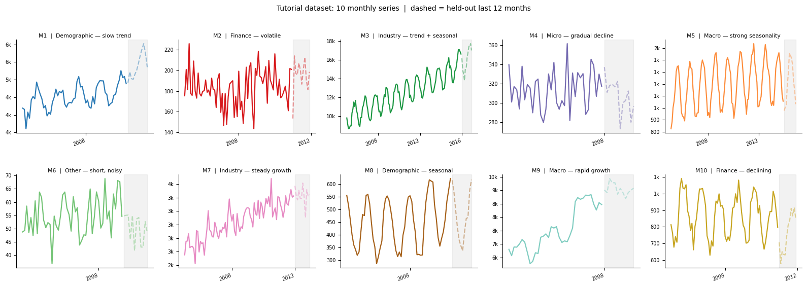
The ten series in the tutorial dataset. Notice how they differ in scale (M3 reaches into the tens of thousands while M6 stays below 70), trend direction (M9 grows rapidly, M4 declines), and seasonal amplitude (M8 is dominated by seasonality while M2 shows very little). This variety is intentional — it mirrors the kind of heterogeneity you would see in a real panel of research series, and it is why AutoGluon’s multi-model approach is useful here.
All code, explanatory notes, and exercises live in the companion notebook. Click the badge to open a temporary Colab session, then click “Copy to Drive” to save your own copy.
![]()
Note
AutoGluon’s medium_quality preset includes Chronos-2 and Temporal Fusion Transformer, but a known compatibility issue between Colab’s pre-installed PyTorch version and torchvision causes these two models to be skipped automatically on Colab. The rest of the workflow runs normally. Step 11 in the notebook, which runs Chronos-2 as a standalone zero-shot predictor, will also not complete on Colab for the same reason. If you want to run the full model list, you will need a local environment with Python 3.10 or 3.11 and torch 2.4.x. See AutoGluon’s install guide for setup instructions.
The Core Call
The forecasting workflow is three steps: create the predictor, call fit(), call predict().
from autogluon.timeseries import TimeSeriesPredictor

predictor = TimeSeriesPredictor(
    prediction_length=12,
    target="target",
    eval_metric="MASE",
    path="autogluon_ts_model"
).fit(
    train_data,
    time_limit=120,
    presets="medium_quality"
)
prediction_length=12 means you want forecasts 12 steps ahead. For monthly data, that is one year. eval_metric="MASE" tells AutoGluon which metric to optimize and rank models by. Two minutes is enough for a first feasibility pass.
Reading the Leaderboard
The time series leaderboard looks similar to the tabular one. Every model that ran is ranked by the evaluation metric, with higher always meaning better (AutoGluon flips the sign on error metrics to enforce this convention). You will typically see a mix of classical models, tree-based models, and the ensemble near the top.
One pattern worth watching: if SeasonalNaive ranks near the top, your series may have strong seasonal structure but limited additional signal for complex models to capture. If deep learning models trail far behind the classical methods, you likely have too few observations for them to learn effectively. These are useful signals for your next modeling decision, not failures of the tool.
Understanding MASE
MASE (Mean Absolute Scaled Error) is the default evaluation metric and the one used in most forecasting benchmarks [Hyndman and Athanasopoulos, 2021]. The key intuition is that it compares your model against a naive seasonal baseline, specifically a forecast that repeats the last observed seasonal value. A MASE of 1.0 means your model performs exactly as well as that naive baseline. Below 1.0 means you are beating it. Above 1.0 means the model has not learned much useful from the data.
Because MASE is scale-free, it does not depend on the units of your target variable, which makes it especially useful when you have multiple series with different scales.
AutoGluon reports it as a negative number in the leaderboard (so that higher is always better). A leaderboard value of -0.82 corresponds to a MASE of 0.82, meaning the model is 18% better than the seasonal naive baseline.
Other metrics worth knowing: SMAPE (symmetric mean absolute percentage error) if you want something easier to explain to collaborators, and WQL (weighted quantile loss) if you care about the accuracy of your uncertainty estimates rather than just the point forecast.
What the Forecast Output Looks Like
Like tabular prediction, predict() returns the best model’s output by default — usually the WeightedEnsemble. If you want a specific model’s forecast, pass its name from the leaderboard using the model= argument. What differs is the output format. Rather than a single predicted value per row, you get a DataFrame with one row per time step per series, and multiple columns for different quantile levels. By default you get the 10th, 50th, and 90th percentiles:
                        0.1      0.5      0.9
item_id  timestamp
M1       2023-01-01    112.3    118.7    124.9
         2023-02-01    109.8    116.2    122.7
         ...
The 50th percentile is your point forecast. The range between the 10th and 90th percentiles is an 80% prediction interval: in a well-calibrated model, the true future value should fall within this range about 80% of the time. Visualizing this interval alongside the historical data is one of the most informative things you can do with a forecast. The width of the interval tells you how confident the model is and how that confidence changes over the forecast horizon.
Practical Notes
Short series. Most models need a history length meaningfully longer than the forecast horizon. A rough rule of thumb is that your history should be at least two to three times longer than prediction_length. If you have 15 monthly observations and want a 12-month forecast, deep learning models will struggle and classical methods are your best option.
Missing observations. AutoGluon handles missing values natively without requiring you to impute them first. If your series has gaps, you can pass the data in as-is.
Irregular time intervals. AutoGluon infers the frequency of your series automatically from the timestamps. If your timestamps are not evenly spaced, you will need to either regularize them or resample to a fixed frequency before passing data in.
Single series. If you have only one series, you can still use TimeSeriesPredictor by setting item_id to a constant value for all rows. Classical and Chronos models work well in this setting.
Covariates. If you have external variables that are known in advance for the forecast period, such as seasonal indicators, treatment assignments, or scheduled events, you can pass these as known_covariates. Models that support covariates (like Temporal Fusion Transformer) will incorporate them automatically. The AutoGluon in-depth forecasting tutorial covers this in detail.
Frequently Asked Questions
How is this different from using the forecast package in R?
The R forecast package gives you precise control over a single model, usually ETS or ARIMA, with rich diagnostic tools [Hyndman and Athanasopoulos, 2021]. AutoGluon trades that control for breadth: it runs many model families automatically and lets you compare them. The two approaches are complementary. AutoGluon is useful for a quick feasibility pass across many models; a dedicated tool like R’s forecast package is better when you have chosen a direction and want to go deeper with one model.
My dataset has hundreds of series. Will this take forever?
With time_limit=120 and presets="medium_quality", two minutes is usually enough for a first pass even on moderate-sized panels. If you have a large panel and limited compute, try presets="fast_training" for a first run. It focuses on faster models and gives you a leaderboard quickly.
Should I fine-tune Chronos rather than just using zero-shot?
For a feasibility test, zero-shot Chronos is usually sufficient. If the results look promising and you want to squeeze more accuracy, AutoGluon supports fine-tuning Chronos on your specific dataset. Fine-tuning is most worthwhile when you have at least a few hundred observations and your series have patterns that differ from what general pretraining data covers [Ansari et al., 2024].
My outcome is binary — can I still use AutoGluon?
It depends on what your question actually is. If you are asking “when will this event occur,” that is a survival analysis or time-to-event problem, and TimeSeriesPredictor is not the right tool for that.
But in many research contexts — neuroimaging work especially — the question is different. If you have segmented your time series into epochs and want to classify each epoch as condition A or condition B, that is a tabular classification problem, not a forecasting problem. You extract features from each epoch (band power, peak amplitude, windowed statistics, whatever is appropriate for your signal), put those in a DataFrame, and run TabularPredictor. This works well for EEG and fNIRS data where the goal is decoding a mental state or condition label from a fixed time window. TimeSeriesPredictor was never the right entry point for that kind of work — TabularPredictor is.
Research Considerations
The same cautions from the tabular chapter apply here, and time series adds a few of its own.
Temporal leakage is easy to miss. Beyond the train/test split, watch for features derived from the target across time. If you include a rolling average of your target as a covariate, and that average incorporates future observations, you have a leak. AutoGluon does not protect you from leakage in covariates you supply.
Stationarity and structural breaks. Classical models like ARIMA assume the statistical properties of the series are stable over time. If your data contains a regime change, such as a policy shift, an intervention, or an external shock, a model trained before the break may forecast poorly after it. Looking at your raw series before modeling is always worth the time.
Forecasts are not causal. A model that forecasts well does not tell you why the series behaves as it does. If the goal is to evaluate an intervention or understand a mechanism, forecasting tools alone are not sufficient.
On data privacy. For any data covered by HIPAA or other governance policies, run in an approved institutional environment or a local installation, and do not upload sensitive data to a public Colab notebook. Chapter 13 covers computing options in more detail.
If You’re at U-M
Approved options include Great Lakes for general sensitive workloads and Armis2 for HIPAA-covered data. See AI Resources at the University of Michigan.
Last reviewed: April 2026. Tool-specific content in this chapter refers to AutoGluon 1.x. If you notice outdated content, open an issue on GitHub.
References
Oleksandr Shchur, Ali Caner Turkmen, Nick Erickson, Huibin Shen, Alexander Shirkov, Tony Hu, and Yuyang Wang. AutoGluon-TimeSeries: AutoML for probabilistic time series forecasting. arXiv preprint arXiv:2308.05566, 2023. URL: https://arxiv.org/abs/2308.05566.
Rob J. Hyndman and George Athanasopoulos. Forecasting: Principles and Practice. OTexts, Melbourne, Australia, 3rd edition, 2021. Accessed 2026-03-04. URL: https://otexts.com/fpp3/.
Abdul Fatir Ansari, Lorenzo Stella, Caner Turkmen, Xiyuan Zhang, Pedro Mercado, Huibin Shen, Oleksandr Shchur, Syama Sundar Rangapuram, Sebastian Pineda Arango, Shubham Kapoor, Jasper Zschiegner, Danielle C. Maddix, Michael W. Mahoney, Kari Torkkola, Andrew Gordon Wilson, Michael Bohlke-Schneider, and Yuyang Wang. Chronos: learning the language of time series. Transactions on Machine Learning Research, 2024. URL: https://openreview.net/forum?id=gerNCVqqtR.
Spyros Makridakis, Evangelos Spiliotis, and Vassilios Assimakopoulos. The M4 competition: 100,000 time series and 61 forecasting methods. International Journal of Forecasting, 36(1):54–74, 2020. doi:10.1016/j.ijforecast.2019.04.014.